Multiple comparisons in a regression framework

Gordon Feld posted a comparison of results from a repeated measures ANOVA with paired samples t-tests.

Using Stata, I wondered how these results would look in a regression framework. For those of you who want to replicate this: I used the data provided by Gordon. The do-file is here. Because wordpress does not accept .do files you will have to rename the file from .docx to .do to make it work. The Stata commands are below, all in block quotes. The output is given in images. In the explanatory notes, commands are italicized, and variables are underlined.

A pdf of this post is here.

First let’s examine the data. You will have to insert your local path at which you have stored the data.

. import delimited “ANOVA_blog_data.csv”, clear

. pwcorr before_treatment after_treatment before_placebo after_placebo

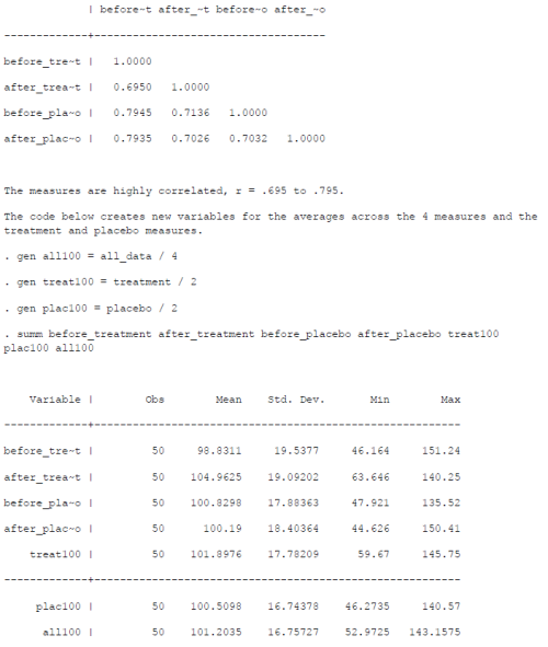
These commands get us the following table of correlations:

There are some differences in mean values, from 98.8 before treatment to 105.0 after treatment. Mean values for the placebo measures are 100.8 before and 100.2 after. Across all measures, the average is 101.2035.

Let’s replicate the t-test for the treatment effect.

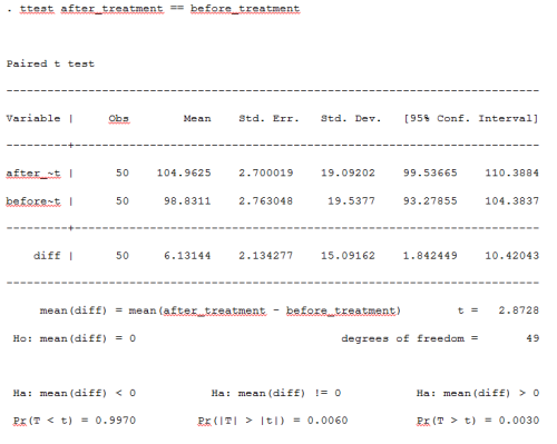The increase in IQ after the treatment is 6.13144 (SE = 2.134277), which is significant in this one-sample paired t-test (p = .006). Now let’s do the t-test for the placebo conditions.

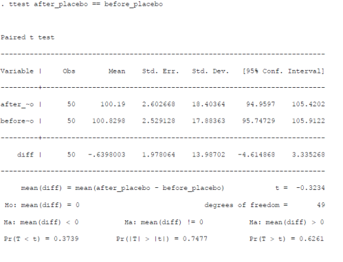
The decrease in IQ after the placebo is -.6398003 (SE = 1.978064), which is not significant (p = .7477).

The question is whether we have taken sufficient account of the nesting of the data.

We have four measures per participant: one before the treatment, one after, one before the placebo, and one after.

In other words, we have 50 participants and 200 measures.

To get the data into the nested structure, we have to reshape them.

The data are now in a wide format: one row per participant, IQ measures in different columns.

But we want a long format: 4 rows per participant, IQ in just one column.

To get this done we first assign a number to each participant.

. gen id = _n

We now have a variable id with a unique number for each of the 50 participants.
The Stata command for reshaping data requires the data to be set up in such a way that variables measuring the same construct have the same name.
We have 4 measures of IQ, so the new variables will be called iq1, iq2, iq3 and iq4.

. rename (before_treatment after_treatment before_placebo after_placebo) (iq1 iq2 iq3 iq4).

Now we can reshape the data. The command below assigns a new variable ‘mIQ’ to identify the 4 consecutive measures of IQ.

. reshape long iq, i(id) j(mIQ)

Here’s the result.

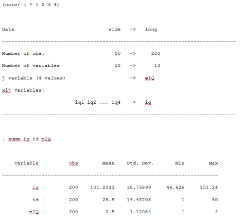
We now have 200 lines of data, each one is an observation of IQ, numbered 1 to 4 on the new variable mIQ for each participant. The variable mIQ indicates the order of the IQ measurements.

Now we identify the structure of the two experiments. The first two measures in the data are for the treatment pre- and post-measures.

. replace treatment = 1 if mIQ < 3 (100 real changes made) . replace treatment = 0 if mIQ > 2
(100 real changes made)

Observations 3 and 4 are for the placebo pre- and post-measures.

. replace placebo = 0 if mIQ < 3 (100 real changes made) . replace placebo = 1 if mIQ > 2
(100 real changes made)

. tab treatment placebo

We have 100 observations in each of the experiments.

OK, we’re ready for the regressions now. Let’s first conduct an OLS to quantify the changes within participants in the treatment and placebo conditions.

The regression shows that the treatment increased IQ by 6.13144 points, but with an SE of 3.863229 the change is not significant (p = .116). The effect estimate is correct, but the SE is too large and hence the p-value is too high as well.

. reg iq mIQ if placebo == 1

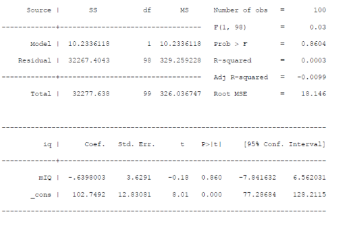
The placebo regression shows the familiar decline of .6398003, but with an SE of 3.6291, which is too high (p = .860). The SE and p-values are incorrect because OLS does not take the nested structure of the data into account.

With the xtset command we identify the nesting of the data: measures of IQ (mIQ) are nested within participants (id).

. xtset id mIQ

First we run an ’empty model’ – no predictors are included.

. xtreg iq

Here’s the result:

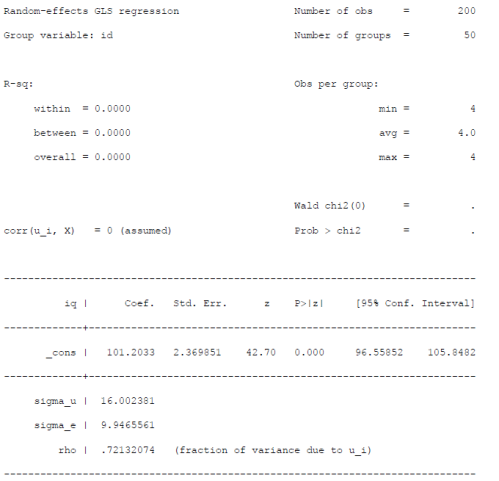
Two variables in the output are worth commenting on.

1. The constant (_cons) is the average across all measures, 101.2033. This is very close to the average we have seen before.
2. The rho is the intraclass correlation – the average correlation of the 4 IQ measures within individuals. It is .7213, which seems right.

Now let’s replicate the t-test results in a regression framework.

. xtreg iq mIQ if treatment == 1

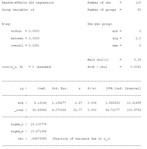
In the output below we see the 100 observations in 50 groups (individuals). We obtain the same effect estimate of the treatment as before (6.13144) and the correct SE of 2.134277, but the p-value is too small (p = .004).

Let’s fix this. We put fixed effects on the participants by adding , fe at the end of the xtreg command:

. xtreg iq mIQ if treatment == 1, fe

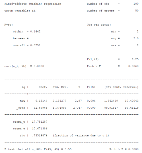
We now get the accurate p-value (0.006):

Let’s run the same regression for the placebo conditions.

. xtreg iq mIQ if placebo == 1, fe

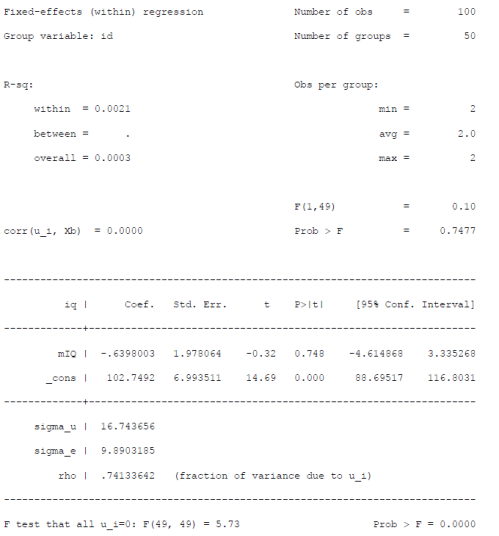
The placebo effect is the familiar -.6398003, SE = 1.978064, now with the accurate p-value of .748.